Big-O Time & Space Analysis

Nov 08, 2023

Introduction

Big O Notation is the language we use for talking about how long an algorithm takes to run.

We can compare it to different algorithms or functions using Big O and say which one is better than the other when it comes to scale, regardless of our computer differences.

And we can measure Big O like this.

This may look really confusing at first, if it’s the first time you’re seeing this diagram, but don’t worry, by the end of this article, this is going to make sense and you’re going to be completely fluent in this.

When we talk about Big O and scalability of code, we simply mean when we grow bigger and bigger with our data how much does the algorithm or function slow down? As the list of elements in the input increases how many more operations do we have to do? That’s all it is.

And Big O allows us to explain this concept. Different functions have different Big O complexities — that is the number of operations can increase really fast like O(N²), which is not good, you can see that it’s in the red spectrum and things that are quite good actually, and don’t increase as much, like O(logN).

And we’re going to look at examples of different ones and how to actually measure this and what this entire notation means. But just remember this point, when we talk about Big O and scalability of code, we simply mean when we grow bigger and bigger with our input, how much does the algorithm slow down? The less it slows down, the better it is.

What is Big O?

Imagine you’re at a concert, and you’re trying to find your friend, Bob, in a crowd.

One way you might do this is by going through each person in the crowd one by one, asking, ‘Are you Bob?’. This, in Big O terms, would be O(N), where N is the number of people in the crowd. The more people there are, the more time it takes to find Bob. This is known as Linear Time Complexity.

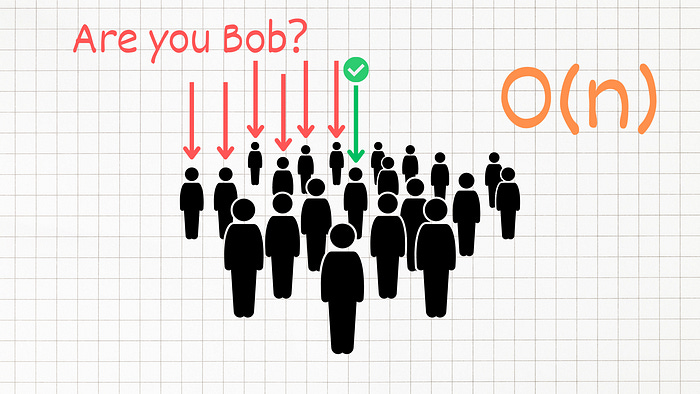
Now, let’s say you could clone yourself, and each clone could also clone themselves, and so on, until there are as many of you as there are people in the crowd. You could then ask everyone at the same time, ‘Are you Bob?’ It would only take a moment to find Bob. This scenario represents O(1) or Constant Time Complexity. Regardless of the crowd’s size, it takes the same amount of time to find Bob.

As you can see, different approaches result in different time complexities, and that’s what Big O notation helps us to quantify.

Big O notation is a way to express how fast an algorithm is. You can think of it like the “speed limit” of a function or algorithm. The smaller the Big O, the faster the algorithm runs.

Different Complexities Explained

Let’s look at all types of time complexities that we have on this chart.

Imagine you’re in a room with a hundred boxes and you’re tasked with finding a specific item. Now, think about how long it would take you to find that item if it were in the first box you checked, versus if it were in the last box.

That’s essentially what we’re dealing with here — best-case versus worst-case scenarios.

O(1)

First up, we have O(1), also known as constant time complexity. This is the ideal scenario where it takes the same amount of time to compute something, regardless of the input size. There are no loops involved here; it’s as if you knew exactly where that item was in the room.

function constantTime(array) {
  return array[0];
}

No matter the size of our array, we are only interested in one specific element. This operation will always take the same amount of time, hence O(1).

O(log N)

Next up is O(log N), or logarithmic time complexity. This is typically seen in searching algorithms, like Binary Search. Imagine our room full of boxes again, but this time, every step you take eliminates half of the remaining boxes. You’re efficiently zoning in on your target until you find the item.

function binarySearch(array, value) {
  let start = 0;
  let end = array.length - 1;
  
  while (start <= end) {
    let middle = Math.floor((start + end) / 2);
    if (array[middle] === value) {
      return middle;
    } 
    else if (array[middle] < value) {
      start = middle + 1;
    }
    else {
      end = middle - 1;
    }
  }
  return -1;
}

In this Binary Search, for each step, we’re reducing our problem size by half. Hence, it’s an O(logN) complexity.

O(N)

Then, we have O(N), known as linear time complexity. This is like checking each box one by one until you find your item. It’s pretty straightforward: as your input grows, the time it takes grows linearly.

function linearTime(array) {
  array.forEach(function(item) {
    console.log(item);
  });
}

For every item in the array, we are performing an operation. Hence, the time it takes scales linearly with the number of items.

O(N logN)

For more complex operations, we have O(N logN), or log-linear time complexity. This is usually the case for sorting operations. It’s like having to not only find specific items but also arrange them in a certain order.

This often refers to efficient sorting algorithms like merge sort or quick sort. Here’s an example of the merge sort:

function mergeSort(array) {
  if (array.length < 2) {
    return array;
  }
  let middle = Math.floor(array.length / 2);
  let left = array.slice(0, middle);
  let right = array.slice(middle);
  
  return merge(mergeSort(left), mergeSort(right));
}

This is a merge sort algorithm. It divides the problem down and then merges the solutions, resulting in an O(N log N) complexity.

O(N²)

Then comes O(N²), or quadratic time complexity. This is seen when every element in a set needs to be compared to every other element. Think of it like this: for every box in our room, you have to open it and compare it with every other box.

function quadraticTime(array) {
  for (let i = 0; i < array.length; i++) {
    for (let j = 0; j < array.length; j++) {
      console.log(array[i], array[j]);
    }
  }
}

Here, for each element in the array, we are looping through the entire array again. This gives us N² operations.

O(2^N) & O(N!)

O(2^N), or exponential time complexity, and O(N!), or factorial time complexity, which are at the higher end of our complexity spectrum, often seen with recursive algorithms or when adding a loop for every element.

For instance, this function recursively calculates the Fibonacci sequence, but it does so inefficiently by recalculating lower numbers multiple times.

function fibonacci(num) {
  if (num <= 1) return num;
  return fibonacci(num - 2) + fibonacci(num - 1);
}

This leads to a lot of extra calculations, hence the exponential time complexity.

This other function generates all permutations of an array.

function permutation(array, start = 0) {
  if (start >= array.length) {
    console.log("[" + array.join(", ") + "]");
  }
  for (let i = start; i < array.length; i++) {
    [array[start], array[i]] = [array[i], array[start]];
    permutation(array, start + 1);
    [array[start], array[i]] = [array[i], array[start]];
  }
}

For each element, it swaps the element with each element (including itself) and then recurses for the remaining elements. Hence, it has factorial time complexity.

What causes time in a function

Now, let’s discuss what could cause time in a function. This could be the result of operations like addition or subtraction, comparisons like greater than or less than, looping constructs like ‘for’ or ‘while’, and calling outside functions.

It’s important to remember a few rules when dealing with Big O Notation:

Rule 1: Always consider the worst-case scenario.
Rule 2: Remove constants. We’re more interested in how our algorithm grows, not the precise details.
Rule 3: Different inputs should have different variables. So, if you have two different inputs, we’d express it as O(a+b) or O(a * b).
Rule 4: Drop non-dominant terms. When considering the complexity, we focus on the parts that have the most impact.

Space Complexity

Now let’s talk about the space complexity.

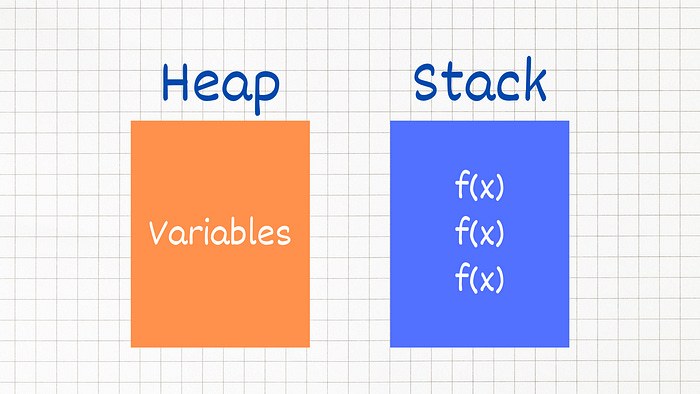
When a program executes it has 2 ways to remember things — the heap and the stack. The heap is usually where we store variables that we assign values for and the stack is where we keep track of our function calls.

Sometimes we want to optimize for using less memory instead of using less time. Talking about memory or Space Complexity is very similar to talking about Time Complexity. We simply look at the total size relative to the size of the input and see how many new variables or new memory we’re allocating.

We also have to consider how much input our function can take, for example, if we are using a ton of space when running our function the memory might overflow.

So what causes space complexity? Here are some factors that contribute to space complexity:

Variables: Variables are used to store data within our code. The size and number of variables can impact the space complexity. For example, if we have an array with “n” elements, it will require “n” units of memory to store all the values.
Data Structures: Data structures like arrays, linked lists, trees, or hash tables can also affect space complexity. The size and complexity of these data structures determine how much memory they consume. For instance, a binary tree with “n” nodes will require space proportional to “n.”
Function Calls: When we call a function, memory needs to be allocated for its execution. This includes storing function arguments, local variables, and return addresses. Recursive functions can have a significant impact on space complexity since each recursive call adds to the memory usage.
Allocations: Dynamic memory allocations, such as creating objects or arrays dynamically using keywords like new or malloc, contribute to space complexity. It's important to manage memory allocations efficiently to avoid excessive memory usage.

Remember, when analyzing space complexity, we follow similar principles as with time complexity:

We consider the worst-case scenario to evaluate the maximum memory usage.
We remove constants and focus on the overall trend.
Different inputs should have different variables in the complexity expression.
We drop non-dominant terms to focus on the main contributors to space usage.

Summary

That’s all you need to know about time and space complexities to estimate the complexities of your functions. I hope this diagram now makes more sense to you and it was easy to follow.

Below I’ll attach some more resources in case you’d like to dive deeper into Big O.

Resources

Big O cheat sheet — bigocheatsheet.com
Freecodecamp article — https://www.freecodecamp.org/news/big-o-cheat-sheet-time-complexity-chart/
Sorting algorithms and data structures — https://cooervo.github.io/Algorithms-DataStructures-BigONotation/
Sorting algorithm visual explanations — https://www.toptal.com/developers/sorting-algorithms
Thanks for reading! Subscribe for free to receive new posts and support my work.

Hayk Simonyan

Discussion about this post